Executive Summary
Catching very-high-energy gamma rays from the ground does not involve looking at the sky directly. A gamma ray hits the atmosphere, produces a Cherenkov flash lasting a few nanoseconds, and a large mirror collects that flash onto a camera. For forty years this field has improved performance in one way: by building bigger mirrors. Researchers at the Max Planck Institute for Physics and the Technical University of Munich left the mirror alone and went after the data-processing rules that sit in front of it.
They simulated a small telescope with a 5-metre dish, treated each event as a 25.6-nanosecond movie, and passed the whole thing to a video vision transformer. No calibration, no cleaning, no parameterization. Measured against an optimized standard analysis on the same simulated events, the detection threshold fell from 0.22 TeV to 0.07 TeV. On benchmarks where the two analyses overlap, though, such as energy resolution, the standard analysis still leads.
These results come from a Monte Carlo simulation of an idealized virtual telescope, not from an observing campaign. The authors write themselves that the absolute numbers are upper bounds. This article keeps that condition in view and asks how far the claim can be read: that the limit sat not in the hardware but in a front-end processing rule nobody had reason to question for forty years.
Key figures
Source: Jobst et al. (2026), arXiv:2608.31148, Table 5 and §1
0.22 → 0.07 TeV
Energy detection threshold
Two analyses on identical simulated events, a factor of 3.1 lower
3.3×
Effective collection area
At 0.2 TeV, from 0.32 to 1.05×10⁵ m², with the same mirror
460,800 → ~10
Values surviving per event
What the standard pipeline hands to the reconstruction stage
0.28 vs 0.32
Where the transformer loses
Energy resolution at 0.2 TeV, standard analysis ahead, lower is better
What Cleaning Erases from a Few Dozen Photons
Very-high-energy gamma rays are absorbed in the atmosphere before they reach the ground. An Imaging Atmospheric Cherenkov Telescope (IACT) therefore does not see the gamma ray itself but the particle shower it triggers in the air. The relativistic charged particles in that shower emit Cherenkov light in a narrow forward cone, a flash of a few nanoseconds that illuminates a light pool roughly 120 metres in radius at ground level. Large segmented mirrors focus that light onto a pixelated camera with high time resolution. The technique matured in the late 1980s with the first detection of the Crab Nebula, and more than 220 very-high-energy sources have been detected with it since.
In the camera the shower appears as an elongated ellipse, a few photons per pixel. Its orientation, shape and brightness encode the direction and energy of the gamma ray, and they also carry what is needed to tell it apart from showers started by hadronic cosmic rays, which are four orders of magnitude more abundant. The dominant noise here is not electronic. It is the sky itself: the diffuse night-sky background from unresolved stars, airglow and scattered light keeps arriving at the camera.
So the first job of the standard analysis is to separate signal from background. Each pixel waveform is reduced to two values, a charge and an arrival time. The resulting image is then cleaned: pixels judged to be dominated by the night-sky background are set to zero. The surviving pixels are reduced to a handful of variables such as length, width, size, centroid and orientation, and random forests estimate the energy, the direction and the particle type from those variables alone. The pipeline rests on a high compression factor, as the paper puts it. A modern camera with thousands of pixels sampled at a few GHz records on the order of 100,000 values per event; the Hillas parameterization keeps on the order of ten.
For bright events that compression is sensible. The image is large, well contained and geometrically simple, so ten variables hold it. The trouble is at the low end. The image grows faint, and a few tens of photoelectrons scatter over a handful of pixels. The cleaning removes most of the signal along with the background, and the surviving pixels no longer support a stable parameterization. The introduction of the paper sums the situation up this way.
"The low-energy performance of an IACT is therefore not just determined by the physical mirror collection area, but also by the capabilities of the analysis chain to efficiently use all recorded information."
That sentence is the hypothesis the rest of the paper sets out to test, and the discussion section restates it as a result: the low-energy performance of a small, stand-alone IACT is limited by the analysis, not by the aperture. Which moves the problem from the hardware budget to the pipeline.
The Mirrors Grew for Forty Years. The First Stage Stayed in 1985.
The back end of this pipeline has kept changing. Static quality cuts gave way to dynamic ones, and the random forests and boosted decision trees used for event classification gave way to neural networks. The front end did not change. The paper states that the low-level part has remained essentially unchanged since the image parameterization introduced by Hillas in 1985. That is 41 years as of 2026, or four decades in the wording of the abstract.
There had been attempts on the front end before. The prior work the paper reviews mostly swapped one stage of the standard chain for deep learning, and took calibrated and usually cleaned images as input. How much the cleaning step affects performance has itself been studied explicitly. More recently, a residual CNN was applied directly to the pixel waveforms of CTAO's LST-1, demonstrating that the temporal structure is usable by a network. Those waveforms were still calibrated, the standard image-cleaning mask was still applied, and the authors of that work noted that the computational cost was too high to propose it as a replacement for the routine analysis chain.
So the novelty this paper claims for itself narrows to two things: the first application of a transformer architecture to IACT data, and the first reconstruction to operate on the raw waveform cube with neither calibration nor cleaning applied.
The way to improve performance, meanwhile, was to grow the reflector. From the 10 metres of Whipple to the 17 of MAGIC, then the 28 of H.E.S.S. and the 23 of CTAO's Large-Sized Telescope. Stereoscopic observation, several telescopes viewing the same shower from different angles, became standard alongside. Performance rose and so did cost. The paper puts it plainly: the cost of an IACT scales empirically with the mirror diameter to the power of about 3. Double the diameter and the cost goes up eightfold.
Large telescopes carry another burden. Enclosing a big instrument in a dome is not economically practical, so today's IACTs stand permanently exposed to wind and humidity, periodically to rain, dust and snow, and occasionally to volcanic ash. All of that degrades the optical throughput, and the performance with it.
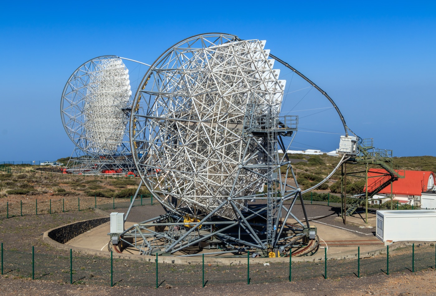
The reason the front end went unquestioned for forty years is not that the rule was wrong. When bright events set the standard, it was the right rule. The compression destroys information only in the regime where the assumption behind it breaks down, in faint events of a few tens of photoelectrons. And that regime is exactly the wall a small telescope has always run into.
One Event as a 25.6-Nanosecond Movie
Rather than use a real telescope, the team designed and simulated a Small Virtual Telescope (SVT). It is a stand-alone instrument with a 5-metre parabolic dish, a square camera of 60×60 pixels, a 6.1-degree field of view and 0.1 degrees per pixel. The site is the CTAO-North location at La Palma, 2,200 metres above sea level. The readout samples at 5 GHz for 128 samples, so one event is a 25.6-nanosecond movie. The trigger fires on an analogue sum over 5×5-pixel regions crossing 10 photoelectrons, and the night-sky background is simulated at 0.15 GHz per pixel.
That movie has shape 128×60×60, which is 460,800 values. The transformer analysis normalizes the tensor by the mode pixel charge of the whole dataset and then feeds it to the network untouched. No calibration, no cleaning, no pedestal subtraction, no parameterization.
3.1Why a video transformer
Before arriving at attention, the team implemented and compared the alternatives on the same data. A convolutional network is the obvious first choice, but convolutions carry a strong locality prior: correlations are learned inside a kernel, and long-range structure has to be built up through depth. An air-shower image is not a local object; its head and tail are strongly correlated. A fixed 3D kernel also treats the temporal axis exactly like the spatial ones, and convolutional architectures are rigid with respect to input size, which is inconvenient when the camera layout is a design variable you may want to optimize later. Recurrent networks handle sequences naturally, but their forget gates lose information over long sequences by construction, a problem for a 128-frame movie in which the informative structure may lie anywhere. Graph networks are the natural tool for irregular detectors, as IceCube showed, but the SVT data are perfectly regular, with square pixels, no dead channels and complete coverage, so the added flexibility buys nothing while the computational cost stays substantial.
What was left was attention. Processing the entire token sequence at once means long-range correlations are present at every layer, and because everything happens in a shared embedding space the architecture accommodates any input that can be tokenized, which keeps it robust to changes in the camera layout.
An event has a temporal axis, so an image vision transformer cannot be applied directly. The team split the movie into three-dimensional patches, tubelets of 20×20 pixels by 2 frames, each embedded by a learned 3D convolution. Pulling frames out separately and concatenating them would break the temporal correlations; tubelets preserve the spatio-temporal structure.
Two architectures were actually run before one was chosen. ViViT-ST, which applies joint spatio-temporal attention, is the most expressive, but on a 128-frame movie its cost grows as the square of the token count. The factorized encoder, ViViT-FE, runs a spatial encoder on each frame independently to produce one token per frame, and a temporal encoder then learns how those tokens evolve. After five epochs on identical data, classification accuracy came out at 80.78% and 80.34%, within half a percentage point, while the wall-clock time for energy-regression training on a single NVIDIA H200 was 1 day 19 hours 58 minutes against 7 hours 39 minutes. With no meaningful accuracy difference and a factor of 5.7 in cost, the factorized encoder won. A broader comparison against convolutional and recurrent baselines, together with the single-frame control that checks whether the temporal information is genuinely used, is reported separately.
The final token feeds a linear head with a four-dimensional output: the energy, two camera-plane coordinates and the class logit. Regression and classification losses differ by orders of magnitude for most of training, so each loss is normalized by its own magnitude, turning the gradients into unit vectors, before the two are combined into a single composite loss. One network performs classification, energy regression and direction regression at once.
3.2The comparison runs against a production pipeline
The weight of a comparison sits in its baseline. The team implemented the analysis chain that CTAO's LST-1 actually uses, in lstchain v0.10.5, and then re-optimized every stage for the SVT, from the calibration integration window through the cleaning thresholds to the random forest settings, using optuna's tree-structured Parzen estimator with 150 trials per stage. This is not a straw man. It is the chain that runs daily on every IACT today, tuned as far as it will go for this telescope.
Applied to the same simulated events, the widest gaps opened on the benchmarks that decide whether an event can be reconstructed at all. The energy threshold dropped from 0.22 TeV to 0.07 TeV, a factor of 3.1, and the lowest energy with usable direction reconstruction dropped from 0.2 TeV to 0.05 TeV, a factor of four. The effective collection area at 0.2 TeV went from 0.32×10⁵ m² to 1.05×10⁵ m², a factor of 3.3. At 0.05 TeV it went from 0.003×10⁵ m² to 0.24×10⁵ m², a factor of 80, which the paper describes as nearly two orders of magnitude. By 1 TeV the two curves converge and the gap narrows to 1.3. Since the trigger, the detector geometry and the input events are identical for both analyses, the difference comes entirely from events that the standard analysis throws away in cleaning and quality cuts and the transformer keeps.
The same pattern holds for telling gamma rays from hadrons apart. The area under the ROC curve converges to 0.94 and 0.99 in the high-energy bins where both analyses have plenty of signal, and the gap widens steadily as the energy falls.
Clearer than the areas are the classifier score distributions. In the standard analysis the gamma-ray and proton gammaness distributions separate cleanly only in the highest energy bins and become indistinguishable below about 0.27 TeV, with both classes piling up at low gammaness. That is what it looks like when cleaning has left the classifier almost nothing to discriminate on. The transformer keeps the two apart below 0.27 TeV and still shows a recognizable difference below 0.13 TeV.
The energy migration matrix shows how the reconstruction collapses. The standard analysis reconstructs almost no event to an energy below 0.1 TeV, even though events with true energies well below that do trigger the telescope. They are either removed by the cleaning, or they survive with too few pixels for a stable parameterization. The matrix therefore broadens into a horizontal band at reconstructed energies of 0.1 to 0.2 TeV, into which events differing by two orders of magnitude in true energy are all piled up. The transformer's matrix follows the diagonal down to a few tens of GeV.
What makes the authors care about this result is where the improvement lands. Transient phenomena such as gamma-ray bursts and flaring active galactic nuclei are brightest and most numerous below 0.5 TeV. That is precisely where the standard analysis of a small telescope collapses.
What These Numbers Do Not Say
Reading this far and concluding that a small telescope actually grew would overstate it. The SVT does not exist. It is a virtual instrument designed to be deliberately simple and idealized: unit mirror reflectivity, 100% quantum efficiency between 260 and 650 nanometres, perfect mirror alignment, zero transit-time spread and a 1-nanosecond FWHM single-photoelectron pulse. Which is why the authors write in §7 that the absolute numbers quoted here are correspondingly upper bounds.
What the paper defends is not the absolute values but the ratio. The same idealizations apply equally to both analyses, so the ratio between them is the claim, and the claim is robust against those idealizations. A first check halved the quantum efficiency: the performance shifted in energy roughly as expected from the reduced photon count, and the transformer's relative advantage held. It proved less sensitive to the change than the standard analysis, in fact, because it does not depend on a cleaning step whose thresholds are tied to the photon yield. A systematic study with realistic optics, wavelength-dependent quantum efficiency and electronic noise is left to a forthcoming paper.
The transformer does not win on every metric. Across the range where both analyses are defined, the standard analysis returns the better energy resolution. At 1 TeV it also leads narrowly on angular resolution.
That deficit varies with energy. The two curves are nearly equal around 0.3 TeV, and the gap only opens up above 0.5 TeV. In the other direction, in the lowest bin where only the transformer has any value at all, the energy resolution rises to about 48%. It fills the place where the standard analysis reconstructs nothing, but the energies it measures there are not precise.
| Benchmark | Standard analysis | Transformer analysis |
|---|---|---|
| Energy threshold | 0.22 TeV | 0.07 TeV |
| Lowest energy with direction reconstruction | 0.2 TeV | 0.05 TeV |
| Energy resolution at 0.2 TeV | 0.28 | 0.32 |
| Energy resolution at 1 TeV | 0.18 | 0.24 |
| Energy quantile ratio at 1 TeV | 5.9 | 2.7 |
| Angular resolution at 1 TeV | 0.10° | 0.11° |
| Angular quantile ratio at 0.2 TeV | 2.7 | 1.7 |
| Effective area at 0.05 TeV | 0.003×10⁵ m² | 0.24×10⁵ m² |
▲ Two analyses on identical simulated events | Resolutions are 68% containment; the quantile ratio is that of the 95% to the 68% containment, for which a Gaussian gives 2. Source: Jobst et al. (2026), Table 5, arXiv:2608.31148
The authors explain the deficit as the price of the composite loss. Binding energy regression, direction regression and classification into one loss means none of them is optimized as hard as it would be alone. The task weight on the regression term was set to unity for these results, and since half the training events are gamma rays and the regression term is masked to those, that places twice the effective weight on classification. Giving the regression term more weight, or replacing the single linear head with a separate head dedicated to the energy, is what the authors call the most direct route to closing the remaining gap. They also note that the model hyperparameters have only been surveyed, not fully optimized.
The quantile-ratio column points the other way. At 1 TeV the ratio of the 95% to the 68% containment of the energy error is 5.9 for the standard analysis and 2.7 for the transformer. A Gaussian gives 2, so the standard analysis carries long tails while the transformer stays between 2.3 and 2.9 across the whole range. It loses on typical accuracy and is badly wrong far less often.
The wall still standing at the lowest energies is the night-sky background. Below about 0.1 TeV the distribution of background photons in the camera overlaps substantially with the signal, and simple thresholding of waveforms does not help. The authors name a learned denoiser applied before the reconstruction network, a diffusion model or a transformer-based alternative, as the next candidate for improvement.
The 0.07 TeV threshold is itself a conservative figure. At the lowest energies the surviving proton background is dominated by Poisson fluctuations in the available simulation statistics, so instead of optimizing the cuts bin by bin the team applied a fixed, deliberately strict gammaness cut of 0.9. With a larger proton sample and per-bin optimization, the threshold would only go lower. And applying any of this to real observations means confronting the data/MC mismatch that limits every simulation-trained IACT analysis. The authors offer domain-adaptation techniques, and the observation that a small telescope can be enclosed in a dome, which stabilizes the optical throughput and thereby improves data/MC agreement directly.
Two Papers Arrived the Same Day, and Neither Went Bigger
A radio astronomy paper posted to arXiv the same day, from a University of Geneva group, has a similar shape. Representations learned by large vision foundation models pretrained on natural images do transfer usefully to astronomical images, and performance on downstream tasks rises with model size, but so does the inference cost. The Geneva team tested the opposite direction: self-supervised pretraining of a 6-million-parameter model on 20,000 unlabeled radio galaxy images.
The pretraining objective was LeJEPA, published in 2025 by Randall Balestriero and Yann LeCun, with SimCLR and BYOL on the same backbone as the comparison group. Across three public classification datasets, the fine-tuned macro F1 scores for LeJEPA ViT-Tiny were 0.72, 0.77 and 0.96, comparable to or slightly above the 0.71, 0.74 and 0.93 of a 22-million-parameter model 3.7 times its size. SimCLR and BYOL at the same 6-million size trailed on all three.
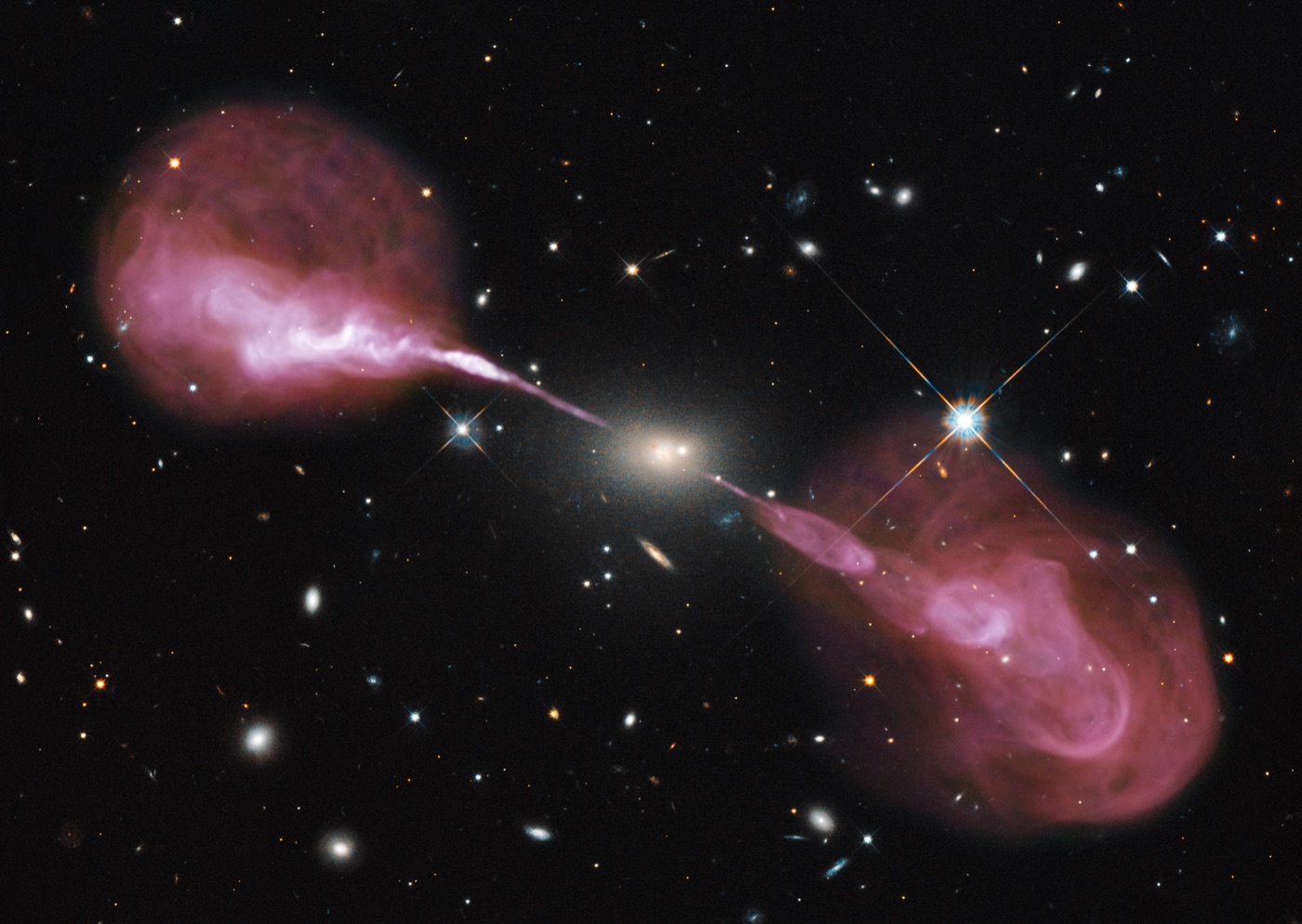
Two things belong alongside that reading. The 22-million-parameter comparison model is itself distilled from a larger teacher, so this is not an experiment against a model with billions of parameters. And with the backbone frozen and only a linear classifier on top, the ranking shifts: the EfficientNet-based LeJEPA variant scored higher on several datasets. Above all, this is a four-page report submitted to a NeurIPS workshop, so its evidentiary weight is not that of the gamma-ray paper, which runs 22 pages with 10 figures and 5 tables. The safer reading is directional: the choice of objective matters about as much as model size.
Narrowed to the front end, the two papers are not easy to set side by side. The RGZ20k images the radio team pretrained on had already been through sigma-clipping, which sets any pixel below 3σ of the image mean to zero. The very kind of front-end rule the gamma-ray paper removed is still in place on the radio side.
Still, the two clearly point in the same direction. One read the raw data it used to discard instead of growing the mirror; the other learned a representation from its own domain observations instead of growing the model. Both chose a representation fitted to their own data over buying something bigger.
The same structure turns up in ordinary data pipelines. The rules that decide what gets aggregated and what gets dropped are usually written around the common, strong-signal cases of the era in which they were designed, much as the Hillas parameterization was designed around bright images. And what disappears first under such a rule is the rare and the weak, which is to say the tail of the distribution. Before layering a new model on top, the question worth asking is not how the model performs but what the storage stage is already erasing.
There is an option available only to organizations that have an answer. §8 of the paper names two implications of this analysis: designing new instruments around transformer-based reconstruction, and improving the reach of existing instruments such as MAGIC, LST and ASTRI by re-analysing their data. The second is possible only where the raw data was kept. Weighing black holes with a ten-year KMTNet archive built to hunt planets, which this blog covered earlier, had the same shape. The observations were long finished; what was new was the way of reading the record.
The picture the paper draws beyond that has more than one telescope in it. Compact telescopes can be domed, robotically operated and solar-powered, which makes arrays of longitudinally distributed telescopes economically feasible. A given source is observable from any one site for at most a few hours per night, so the light curves IACTs produce come in nightly fragments with long gaps. Telescopes spread in longitude could follow the same source continuously as the Earth turns. Variability on timescales of hours to days, where much of the physics of blazars, gamma-ray bursts and compact-object mergers lies, would become accessible at sub-TeV energies as it already is in radio, optical and X-rays.
The new thing in this paper is not the transformer. The video vision transformer itself was proposed in 2021. What changed is what the model was given as input. This is a measurement of what happens when the raw data goes into a slot that had been receiving a summary for forty years.
Editor's Note
Preparing AI-Ready Data is usually understood as labelling and filling in what is missing. This paper reopens a question that comes before that. Is the shape we decided to store in still adequate for the model we now want to use? If the model that the summarization rule was written for is not the model in front of us, the performance ceiling may be sitting in the rule rather than in the model.
References
Primary sources
- 1.Jobst, E., Heckmann, L., Heinrich, L., & Paneque, D. (2026). "The Analysis, not the Aperture: End-to-End Transformer Reconstruction for Imaging Atmospheric Cherenkov Telescopes." arXiv:2608.31148.
- 2.Lastufka, E., Drozdova, M., Kinakh, V., Holotyak, T., Dessauges-Zavadsky, M., Schaerer, D., & Voloshynovskiy, S. (2026). "Learning Radio Astronomical Representations with LeJEPA and Very Small Models." arXiv:2608.30594.
Methods
- 3.Hillas, A. M. (1985). "Cerenkov light images of EAS produced by primary gamma rays and by nuclei." Proceedings of the 19th International Cosmic Ray Conference (La Jolla), Vol. 3, pp. 445–448.
- 4.Arnab, A., Dehghani, M., Heigold, G., Sun, C., Lučić, M., & Schmid, C. (2021). "ViViT: A Video Vision Transformer." arXiv:2103.15691.
- 5.Balestriero, R. & LeCun, Y. (2025). "LeJEPA: Provable and Scalable Self-Supervised Learning Without the Heuristics." arXiv:2511.08544.
Tools and software
- 6.Bernlöhr, K. (2008). "Simulation of imaging atmospheric Cherenkov telescopes with CORSIKA and sim_telarray." Astroparticle Physics 30(3), pp. 149–158.
- 7.Akiba, T., Sano, S., Yanase, T., Ohta, T., & Koyama, M. (2019). "Optuna: A Next-generation Hyperparameter Optimization Framework." KDD 2019, pp. 2623–2631.