Executive Summary
The paper Andrew Gould of Ohio State University posted to arXiv on 26 August 2026 uses no telescope at all. The microlensing records that KMTNet, run by the Korea Astronomy and Space Science Institute at three sites in the southern hemisphere, piled up between 2016 and 2026 stay exactly where they are. What the paper does is calculate how precisely those records could weigh a black hole drifting alone through the Galaxy.
The answer is an Einstein radius error of 0.5 milliarcseconds. That figure holds only across the roughly 12 square degrees watched most intensively; over the 28 square degrees beyond it, the error doubles. What separates the two is not the objects being measured but how often that patch of sky was photographed. And a condition hangs over every one of these numbers: that the systematics peculiar to ground-based observation can be controlled.
So the calculation asks two things at once. What has to be in place for that number to hold? And what had to survive in a collection system designed a decade ago to hunt exoplanets, before it could answer an entirely different question?
Key numbers
The first two numbers say what this calculation believes it can do; the second two say what ground it stands on. The record over 25 years is a single object, and the reprocessing needed to pick out candidates has been finished for one year's worth of data.
Sources: Gould, A. (2026), arXiv:2608.26399 · Segev et al. (2026) MNRAS 546, 1
0.5 mas
Einstein radius error
Across the ~12 deg² monitored most intensively, assuming systematics are controlled
10 mas
Scatter of a single measurement
What the Segev pilot reached at I = 18, the input to this calculation
1
Isolated black holes with a settled mass
OGLE-2011-BLG-0462, out of more than 50,000 microlensing events
2023
The only year re-reduced in full
The TLC re-reduction that candidate selection needs, applied at scale
Not One Hour of New Telescope Time
Gould's paper reports no observations. It photographs no new stars and discovers no new events. What it uses instead is a Fisher analysis, a way of working out in advance how large the errors will be from the observing conditions alone, before any measurement is made. Feed in the number of observations, how they are spread in time, and the precision of a single measurement, and out comes the error on the quantity you finally want.
So what the paper delivers is closer to a map than to a discovery. It takes the KMTNet archive as it already exists and marks how well each region of it can measure. The author is one person, Andrew Gould of the Department of Astronomy at Ohio State University, and the paper is a preprint submitted on 26 August that has not yet been through journal review.
The calculation became possible because of something else. Segev, Ofek, Shvartzvald and colleagues published a pilot study in MNRAS in 2026: the first attempt to pull astrometric time series, records of how a star's position shifts, out of KMTNet's ten-year, roughly 100-square-degree ground-based database, and it reached a usable precision. Gould takes that precision as an input and builds the calculation on top of it. The observing technique belongs to the Segev team; working out what can be done with it is Gould's part.
The last sentence of the abstract states the goal. Combining photometric and astrometric searches, he sets out a practical program for identifying isolated black holes inside the KMTNet database and measuring their masses and distances.
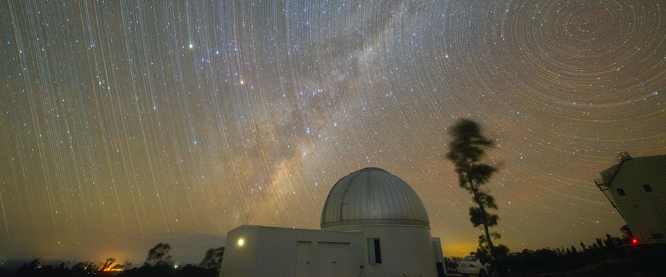
One Isolated Black Hole in 25 Years
A black hole drifting alone, with no companion star, gives off no light. With nothing nearby to swallow, it emits no X-rays either. Microlensing is the only known method for detecting such an object: as the black hole passes in front of a distant background star, its gravity bends the light and the star brightens for a while.
Gould himself predicted in 2000 that on the order of 1% of microlensing events would be caused by black holes. A quarter century later the known events number more than 50,000, and exactly one isolated black hole has been unambiguously identified: OGLE-2011-BLG-0462.
There is only one because settling a mass means measuring two different quantities at the same time. One is the angular Einstein radius, the size of the ring the lens draws on the sky. The other is the microlensing parallax, which shows up as a faint wobble in the light curve as the Earth's orbital motion shifts the vantage point. Know both and the mass and the distance follow together.
Of the two, the parallax is in better shape. It can be measured directly from the same light curve that discovers the event, and it comes out best for long events. Better does not mean easy. Black holes produce long events because they are massive, and that same mass makes their parallax small and therefore hard to measure accurately. Black holes in the Galactic bulge are the worst case. Gould writes that we cannot expect some machine to churn out reliable annual parallax measurements from pipeline reductions of hundreds of events taken with ground-based survey data. Still, the real wall is on the Einstein radius side. More than 100 events now have a measured Einstein radius, but the overwhelming majority came through a single route, the finite-source effect. The light curve is distorted when the background star passes directly over a caustic in the lens structure, and those structures come mostly from binary lenses. Planetary events are the prime example.
For an isolated lens the situation is different. That structure shrinks to a single point, so the chance of the background star crossing it falls to the ratio of the source radius to the Einstein radius. For a lens with an Einstein radius as large as a black hole's, that ratio is below one in a thousand. The larger the Einstein radius, the lower the odds of measuring it.
So other routes opened up. One is to track the tiny shift in the background star's position directly with a high-resolution telescope such as the Hubble Space Telescope. That is how OGLE-2011-BLG-0462 was confirmed. The lens was unusually nearby at about 1.5 kiloparsecs and the black hole was not exceptionally massive at around 8 solar masses, conditions that made the parallax relatively large at 0.095, and even so that single parallax took considerable effort to measure accurately, while the astrometric time series had to run a full decade. The other route is to resolve the two images directly with an interferometer, proposed in 2001, after which it took 25 years for the instruments to become sensitive enough to reach the faint sources involved.
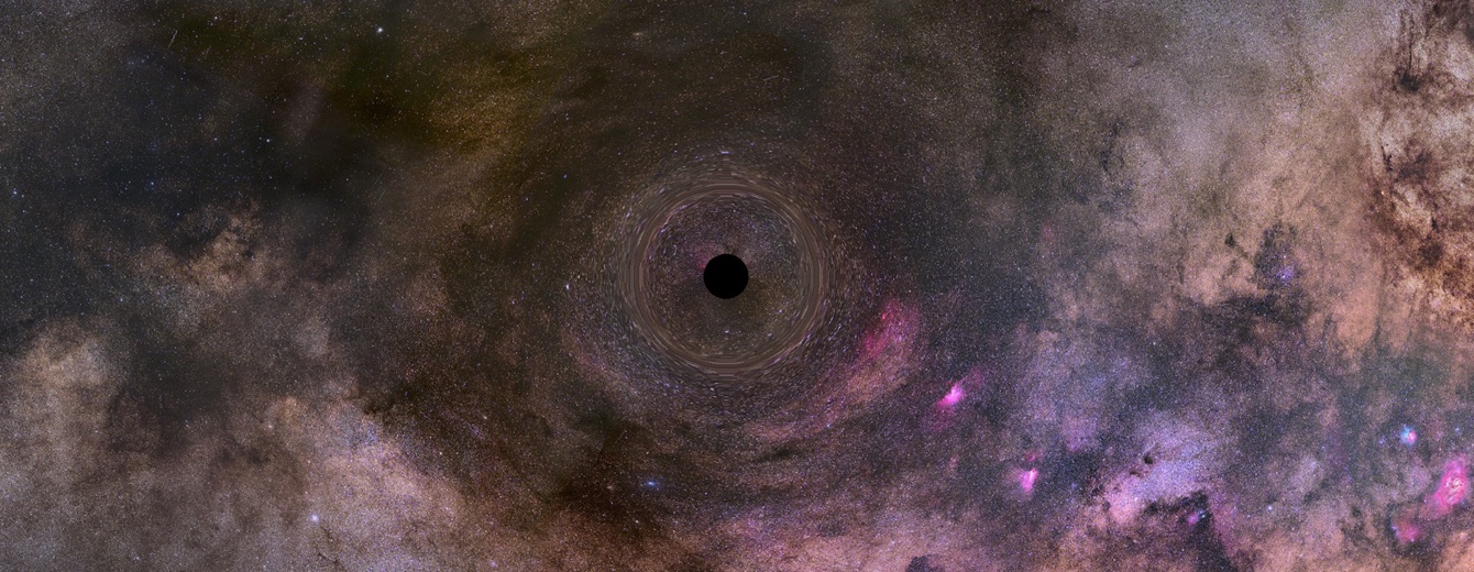
Ten Years from a Planet-Hunting Telescope
KMTNet was not built to weigh black holes. The goal of the project, which the Korea Astronomy and Space Science Institute started in January 2009, is written plainly in its official introduction: to find extrasolar planets by microlensing, and above all to detect Earth-mass planets in the habitable zone.
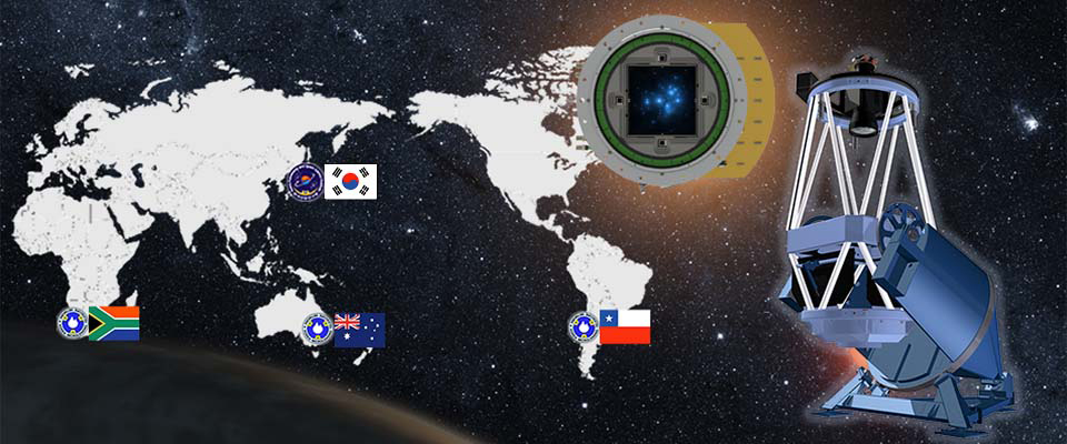
The three-continent layout follows from that goal. Three identical 1.6-metre telescopes sit at three southern sites with widely separated longitudes. The first went in at CTIO in Chile in May 2014, the second at SAAO in South Africa in August, the third at SSO in Australia in November. When it is daytime at one site it is night at another, so the bulge at the centre of the Galaxy can be watched around the clock. Each camera covers two degrees by two degrees, four square degrees in one exposure, and the bulge season runs from 20 February to 22 October, about 46% of the total observing time.
This is the record the Segev team went to work on. Their approach was not to examine events one at a time. It was to build astrometric time series for a large ensemble of stars at once, so that black hole candidates could be searched for independently of the light curves. Running their algorithm on the data from CTIO in Chile, they obtained a scatter of 10 milliarcseconds for a substantial fraction of stars at I = 18 magnitude in KMT field BLG17, which is relatively uncrowded.
So what kind of star sits at I = 18? At the extinctions typical of KMTNet fields, it is a low-luminosity giant. Such stars are certainly less common than the turnoff stars that dominate microlensing statistics, but they are not rare.
Precision That Splits at 12 and 28 Square Degrees
Gould's calculation has six unknowns: two for the background star's position, two for its proper motion, one for the Einstein radius, and one for the direction in which the lens travels. Every observation delivers two position values, one along each axis, and the precision of a single value is fixed at the 10 milliarcseconds the Segev team achieved. Put all of that in, invert the matrix, and the error on the Einstein radius comes out.
The observing schedule is what decides the answer. Across the roughly 12 square degrees where the nominal cadence is four per hour, the rate holds at 40 a day for 40 days around the summer solstice, then falls linearly to 6 a day over the 105 days before that interval and the 95 days after it. That is a 240-day season with a nominal 6,200 observations a year. Weather and equipment problems typically bring it down to 4,800, and Gould scales it back once more to 4,000 usable observations a year, because KMTNet takes data under all conditions, including bright-moon nights.
Under those conditions the Einstein radius error comes out at 0.5 milliarcseconds. For a sense of scale, that is one 7.2-millionth of a degree, about what it takes to resolve a 0.8-millimetre dot in Busan while standing in Seoul. By the paper's own expression, a black hole of 10 solar masses passing with a parallax of 0.05 has an Einstein radius of 4.1 milliarcseconds, so against the quantity being measured, 0.5 milliarcseconds is a little over 12% of it. Other fields carry one extra factor, the square root of four per hour divided by that field's cadence. The 28 square degrees where the error doubles are simply the sky that was watched at a quarter of the cadence.
The same black hole passing in front of a star of the same brightness can be measured twice as precisely or half as precisely depending on which coordinates on the sky it happened to cross. What makes the difference is not a property of the object but an observing plan fixed ten years ago.
The author sets a condition on all of this in the abstract itself. Observing through the atmosphere from the ground still suffers a great deal of systematics, and the precision above holds only where those systematics are controlled.
“Seeing-limited ground-based observations still suffer from a great deal of systematics, but under the assumption that these systematics can be controlled, I find that with this nominal precision, the Einstein radius can be measured with errors σ(θE) ~ 0.5 mas in the most intensively monitored fields (~12 deg2), and hence to twice that value in an additional ~28 deg2 area.”
Gould, A. (2026), arXiv:2608.26399v1, Abstract
He is just as plain about how far the machinery itself reaches. The Fisher analysis assumes that measurement errors are isotropic, and real data will not honour that exactly, if only because the parallactic angle changes over a night and over a season. The calculation is meant to give overall guidance, not to reflect every practical detail.
There is another assumption underneath. The calculation ignores blending, the contamination of a position measurement by light from other stars falling inside the same pixels. For sources around I = 18 the author treats this as a reasonable first approximation: at that brightness the surrounding density of stars of comparable brightness, or even several times fainter, is low enough that experience shows such sources are typically at most weakly blended. He immediately adds a caveat. In any individual case blending can be a moderate, or even a severe, problem, and it must be carefully checked.
The author also writes down where his own calculation stops. There is undoubtedly some floor on the precision reachable for an individual event, perhaps rooted in stellar density, and where that floor lies cannot be settled by calculation. It can only be identified and quantified through the practical work of reducing systematics to a minimum case by case. That does not leave the assumption hanging in mid-air. Gould notes in a footnote that the power spectrum of the astrometric errors in the Segev pilot was roughly flat, which is qualitative support that correlations among the errors can be kept to a minimum in practice.
The Result the Author Called Boring
Having run the calculation across a range of conditions, what the author found most striking was how dull the results were. Section IV opens: “What is most striking about the results reported in Section III is how boring they are.”
Two things show where the dullness lies. The first is timing. For a 60-day event, a typical duration for a black hole candidate, the Einstein radius error stayed nearly flat at around 0.4 milliarcseconds no matter when between 2016 and 2026 the event peaked. The exceptions are 2020, the year lost to Covid-19, and the two edges of the observing window. Even for events peaking in 2020, where the calculation assumes zero observations, the errors are not dramatically worse.
The second is the impact parameter, the measure of how closely the lens grazes past the background star. Within the range in which an event can plausibly be recognised from its light curve, that quantity barely moved the precision either. The reason is geometric. The position shift reaches its maximum at a fixed separation, about 1.4 Einstein radii, the square root of two. Any event that passes closer than that meets the same maximum deviation somewhere along the way.
The observing itself is heavily lopsided. Forty exposures a day pile up in the 40 days around the solstice, and the rate drops to six a day at either end of the season. Even with a schedule tilted that far, events came out with similar errors whenever they occurred.
What remains is brightness. The seasonal dips and bumps in the error are substantially smaller than the factor of about two between an I = 17 source and an I = 18 one. How accurately a single point can be pinned down overwhelms every other condition.
Apart from source brightness, there is no characteristic that marks one event out in advance as a better astrometric candidate than another. That is what boring means in practice. So a black hole search through the archive has to begin by combing the light curves for candidates, and only then investigate those candidates one by one for an astrometric signal. Set against the Segev team's aim of a search independent of the light curves, the light curve comes first again, at least at the stage of measuring the Einstein radius. Gould does not close that door, though. For events passing far enough out that the light curve would barely register them, astrometric sensitivity declines only slowly, which raises the possibility of a purely astrometric search for events with large Einstein radii. He does not pursue it in this paper.
One obstacle stands in the way of that photometric selection. The values the pipeline produces automatically are not enough; what is needed is a labour-intensive reprocessing known as TLC re-reduction. Applying it to a single event is straightforward, but it has only been applied on an industrial scale to one full year of KMTNet events, 2023.
So the procedure the author proposes starts with the re-reduced 2023 data, picking out the events that approximately satisfy a selection criterion. The criterion is the one Gould proposed in 2023 for choosing interferometry targets: a minimum timescale of 50 days for a parallax of 0.025. It eliminates 98.7% of the events produced by solar-mass stars, and 99.8% for the more typical half-solar-mass case, while discarding a 10-solar-mass black hole only if it happens to be moving extremely fast, above 15 milliarcseconds a year in relative proper motion. For the events that survive, re-reducing the 2022 and 2024 data as well and combining them allows a more precise assessment.
For the remaining years, the pipeline values narrow the net. Thresholds on timescale and source brightness promote only the plausible candidates to re-reduction, and the author gives a concrete example. With thresholds of 30 days and magnitude 19 on the 2025 data, 241 events out of 3,348 would require TLC. Raise the timescale threshold to 40 days and the count falls to 174.
What Had to Survive in a Ten-Year-Old Record
The people who put telescopes on three continents in 2014 were not thinking about the astrometric signature of a black hole. What they built was a monitoring system for finding Earth-mass planets in the habitable zone. Twelve years later other researchers opened the same records, asked an entirely different question, and got a result saying that, on paper at least, an answer is available.
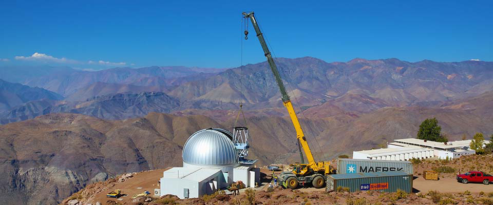
What had to still be there in a ten-year-old record for that reinterpretation to work? Three things.
The first is a record of the collection conditions. Gould's scaling factor only works if the cadence of each field is known. Had there been no record of how many times an hour each patch of sky was photographed, there would be no way to name 12 square degrees apart from 28, and no way to convert the error for the rest. Saying that precision was set by the collection design rather than by the objects is also to say that the precision could be calculated because the collection design survived as a record.
The second is the depth of the time series. A whole year is missing in 2020, and the errors for events peaking that year did not degrade badly, because the other nine years were thick enough to cover the hole. The ability to absorb one year's loss comes out of the span over which the data accumulated.
Depth has a direction as well. Black hole candidates are usually only recognised near peak, or after it. Astrometry, meanwhile, improves greatly if the record starts well before peak. That mismatch is what Gould names as a secondary disadvantage of the astrometric method. The stretch you cannot buy by pointing a telescope at the sky today is exactly that earlier stretch, and the archive already holds it. This is why re-reading an old record is not something a new observation can replace.
The third is being in a state that can be processed again. TLC re-reduction is not a matter of rereading the result tables the pipeline produced; it reduces the data from the start. That requires more than the final product to have survived. KMTNet sends the raw CCD images from all three sites to its data centre in Daejeon for preprocessing, and at that stage the World Coordinate System information is written into the image headers, an entry put there so that positions can be used accurately. That only one year has been re-reduced so far says how expensive this re-reduction is. It also means that had the data been left in no state to re-reduce, candidate selection would never have got off the ground.
This paper has not found a single black hole. It carries an assumption that the systematics of ground-based observation can be controlled, blending has to be rechecked case by case, and the reprocessing needed to pick candidates is finished for one year out of ten. The calculation is done all the same, and everything that went into it has been accumulating for a decade.
Editor's Note
The decision to keep data for a long time is usually treated as a storage question. What this case shows is the question that comes after it. Is a record of what was collected, and under what conditions, being kept alongside the data? Is what survives only the final product, or something that can be processed again? Those two questions are exactly the ones Pebblous keeps running into whenever the subject is AI-Ready Data.
References
Academic papers
- 1.Gould, A. (2026). "Path to Black Hole Astrometric Microlensing from 10-Year KMTNet Database." arXiv:2608.26399.
- 2.Segev, N., Ofek, E. O., Shvartzvald, Y., et al. (2026). "Towards sub-milliarcsecond astrometric precision using high-cadence seeing-limited imaging." MNRAS, 546, 1.
- 3.Sahu, K. C., Anderson, J., Casertano, S., et al. (2022). "An Isolated Stellar-mass Black Hole Detected through Astrometric Microlensing." ApJ, 933, 83.
- 4.Mróz, P., Udalski, A., Gould, A. (2022). "Systematic Errors as a Source of Mass Discrepancy in Black Hole Microlensing Event OGLE-2011-BLG-0462." ApJ, 937, L24.
- 5.Kim, S.-L., Lee, C.-U., Park, B.-G., et al. (2016). "KMTNET: A Network of 1.6 m Wide-Field Optical Telescopes Installed at Three Southern Observatories." JKAS, 49, 37.
Official documentation
- 6.Korea Astronomy and Space Science Institute. "KMTNet, the Korea Microlensing Telescope Network." Introduction, Facilities and Programs pages.