Executive Summary
Nine radio astronomers pulled a single galaxy out of four years of MeerKAT survey observations, put it through two different kinds of compression, and set the results beside a run with no compression at all. Even where the files shrank to roughly a tenth of the original, every physical quantity drawn from that galaxy landed inside the errors. This article follows that result, and the cautions printed right beside it.
The headline number is a spectrum difference below 0.01%. That held with the lossy compressors squeezing the data down to 12–14% of the original. The authors add that the setting goes past what they themselves normally recommend, and that they picked it on purpose so any impact would show.
Sections 1 through 3 follow the paper's own reporting. The questions in sections 4 and 5 belong to this article. If anyone is going to say that data may be cut, someone has to settle first what has to stay the same for the answer to count as unchanged.
Key Figures
Source: Dodson and eight co-authors, Options for Compression of radio interferometry data, arXiv:2609.25988 (posted 22 September 2026).
Below 0.01%
Spectrum difference after compression
That was with the files cut to 12–14% of the original. It held in every case tested
0.7%
Flux gap left by grid-stacking
Nothing is thrown away here, and the gap is still this wide. Image-stacking came to 2.7% in the same comparison
About 10%
The noise floor that rose alongside it
Worst case at tenfold compression. Ease the compression to fourfold and it drops to around 1%
One galaxy
The sample this conclusion rests on
One bright spiral and one weak source. Wider testing is needed, by the paper's own conclusion
The Telescopes Arriving Soon Cannot Keep What They Observe
Three large facilities are arriving in radio astronomy over the next few years: the Square Kilometre Array (SKA), the next-generation Very Large Array (ngVLA), and the Deep Synoptic Array (DSA). The paper puts their gain at roughly an order of magnitude in instantaneous bandwidth, and several orders of magnitude in effective collecting area and therefore in sensitivity. Catching the signal from the era when the first stars lit up, and measuring spectral lines precisely across millions of galaxies, both ride on that gain.
Directly behind the promise comes the constraint. Using that performance means handling volumes of data radio astronomy has never dealt with. For the SKA, the data rate coming out of the correlators is expected to be on the order of one terabyte per second. Long-term storage capacity is limited, so that data has to be buffered on site and processed close to real time.
The constraint bites hardest on observations that stare deep at the same patch of sky across many nights. Traditional imaging sweeps the whole of the original visibility data again on every turn of the deconvolution loop. By the end it is not days' worth but hundreds of days' worth that has to be held all at once. Neither ASKAP nor the SKA, the authors state flatly, can finish a deep neutral hydrogen survey the traditional way within their cost constraints.
So why is there room to compress at all? Interferometric data has a structural quirk. A large share of the measured visibilities is dominated by noise, because the signal from any one bright, localised patch of sky is spread thinly across every baseline, frequency and time sample. On top of that the radio sky is intrinsically sparse, and the brightness temperature of astronomical sources usually runs far below the receiver noise temperature. Volume and information content do not track each other, and that mismatch is the opening.
One Dataset, Two Ways of Cutting It Down
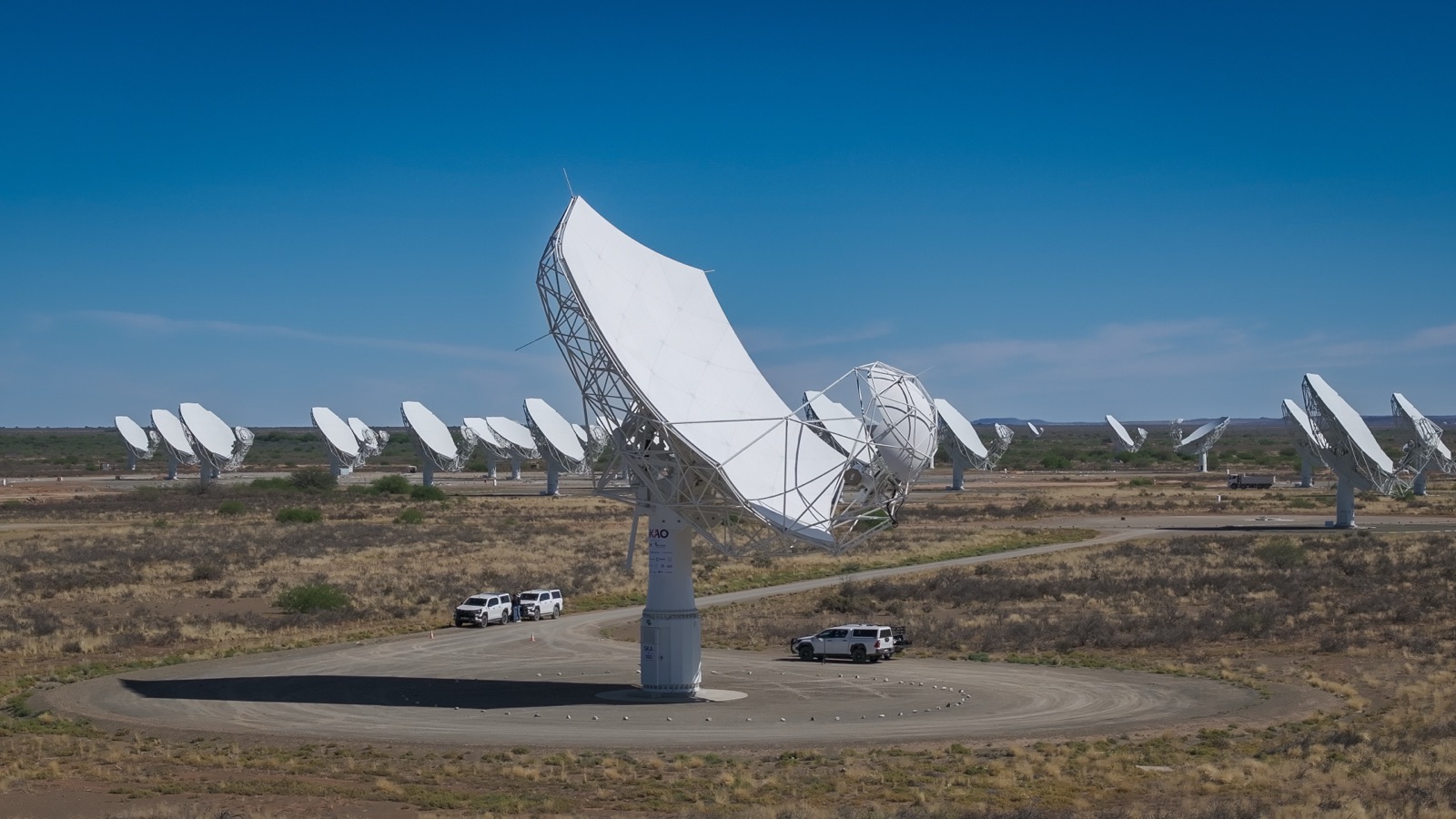
The data on the test bench comes from the MHONGOOSE survey. It is a deep neutral hydrogen survey carried out with South Africa's MeerKAT telescope, covering 30 galaxies within 23 megaparsecs (about 75 million light-years) at 55 hours per galaxy, observed from October 2020 to December 2024. Those 55 hours were not taken in one sitting but split into ten sessions of 5.5 hours. That structure lets a single day be compared against the full stack, which makes it a good set for holding processing methods up against one another.
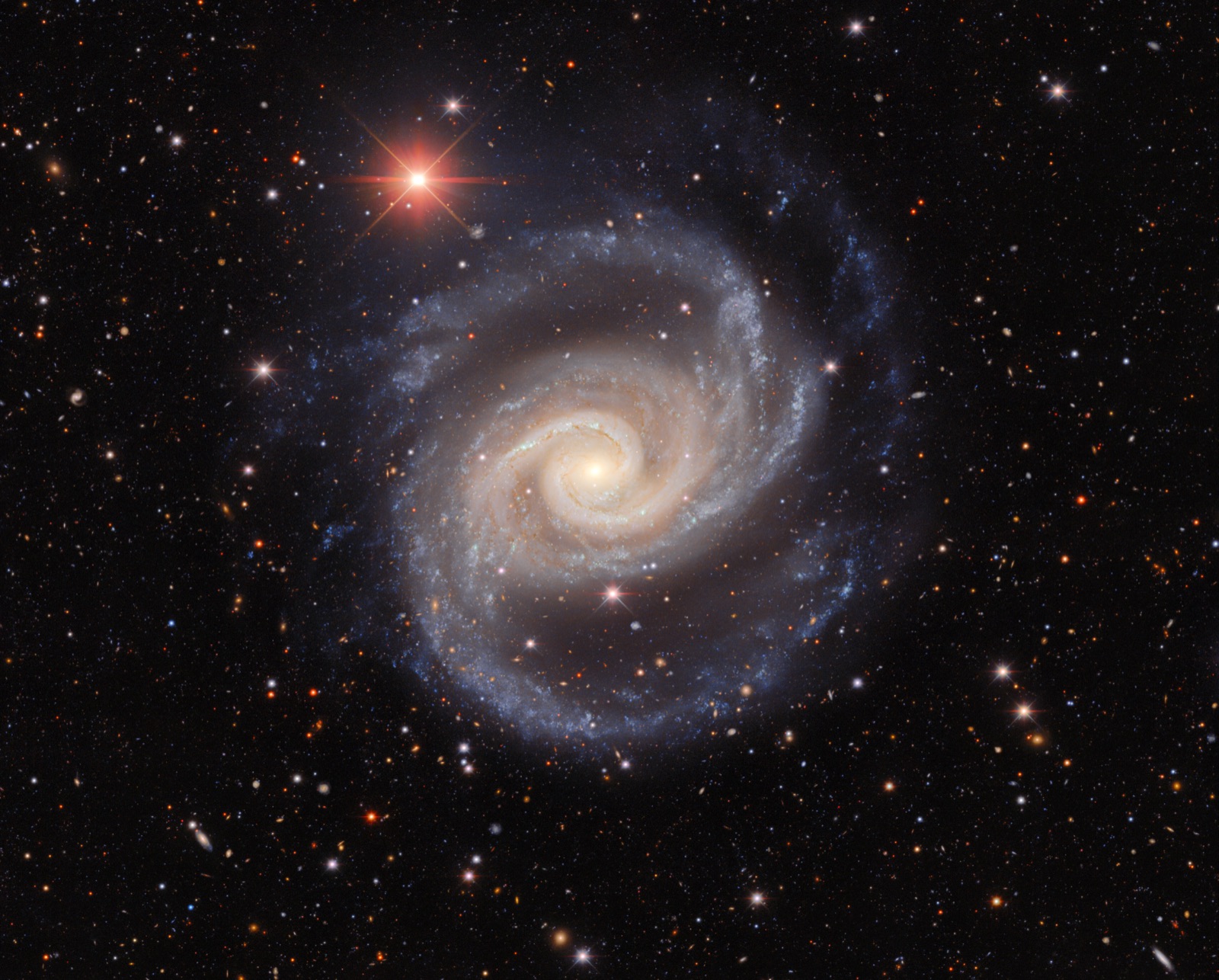
Out of it this work picked NGC 1566, one radio-bright spiral galaxy. It also watched J0422–5455, a much weaker source that happens to fall inside the same frequency coverage. The baseline is the result of traditional processing with no compression, and the question for every other method is how closely it reproduces that baseline.
Establishing the baseline was not simple either. The researchers first ran the same data through the imaging software the MHONGOOSE team had used and through the software they intended to use, and lined the two up. The two tools define Stokes I differently, which left a factor of two between the values, and even after correcting for that a 1% gap in noise and a 10% gap in pixel flux remained. What was left is put down to the different imaging modes, and turning on matching settings reduced the gap without removing it. Measuring a 0.7% difference between methods means keeping a 10% difference between tools out of the comparison. So rather than comparing against the already published images, they took a fresh traditional run made with the same tool as their baseline.
2.1Keeping Every Measurement, Saving Only the Half-Built Image
The first branch is grid-stacking. Each day's visibilities are laid onto the uv grid that same day and stored as residual grids, and once the observing is finished those grids are stacked together for imaging and deconvolution. Nothing is turned into an approximation, so it is lossless, but once the values are on a two-dimensional grid the major cycle can no longer be rerun. That forces each day's processing to produce residuals already close to final.
The value of this method is not only in storage. It does not reduce the amount of computation, but it does let that computation be spread across the whole observing campaign. One epoch took about 10 hours, while processing the same data traditionally in one pass took 34 hours. Nothing was optimised, so both figures should be read as upper bounds. There is also something thrown in. Keep the grids and you can later change the weighting scheme and reconstruct at a different resolution without a significant computing cost.
Even the throw-in has a measurement attached. Re-imaging the same data traditionally at a different weight took around 30 hours; reconstructing from the stored grids took around 5 minutes. Spreading the work out, though, is not the same as having less of it. In the paper's compute comparison, grid-stacking runs 9.9 hours per epoch across ten epochs, while compression followed by traditional processing runs 34 hours once, plus the time to compress and reconstruct. The extra on that second route falls between 0.4 and 3.6 hours depending on the compressor. The peak comes down, and the total goes up.
2.2Fewer Bits per Value, a Smaller Original
The second branch is lossy compression. The original visibilities themselves are shrunk, and everything after that runs as usual. Two different sorts of tool were used. DYSCO fixes how many bits carry each value; here 8 bits and 4 bits were applied, for a fourfold and an eightfold reduction. SZ and MGARD instead take a bound on the allowable error, and the team says it prefers that kind. In radio astronomy the measurement precision is already known from the sensitivity of the instrument, so the noise that compression injects can be set against that precision.
The reason the neutral hydrogen community stays wary of this branch is written down too. Any adverse effect would only surface after thousands of hours of observing, and once introduced, a loss cannot be reversed. Grid-stacking has a doctoral thesis behind it that chased down the fine systematic effects; the equivalent check on lossy compression has not been done, a point made in the same place. This work aims at exactly that gap.
One more method joins the comparison: image-stacking. It is the older approach of saving each day's finished image and averaging at the end, and the paper writes that it is now widely accepted to be a poor option. The judging was handed to SoFiA, an automated source-finding package. Position, line-of-sight velocity, integrated flux, velocity width and the rest are pulled out method by method and placed side by side.
One thing had to be fixed before the comparison would hold. The first imaging run kept the beam shape as it was in the original analysis, but the restored beam turned out slightly different for each method, mixing a difference of method with a difference of beam. So a taper was applied per epoch and per frequency channel until every result carried an identical beam. Measuring the difference between two processing methods requires everything else to be the same, which is the elementary discipline of a controlled comparison.
Nine-Tenths Smaller, and Still the Same Galaxy
Start with the lossy side, where the gaps are strikingly small. MGARD brought the data to 12% and 22% of the original, SZ to 14% and 24%, DYSCO to 12.5% and 25%. Even at the hardest of those settings, the difference across the inner half of the spectrum stayed below 0.01%. At the gentler settings it is nearer 0.001%. Under the table that lists the galaxy's integrated flux, velocity width and neutral hydrogen mass by method, there is one line: all science outcomes are within errors.
The authors themselves do not call this a surprise. The caption of Figure 6 gives the reason in brief. These compressors scatter individual values but are guaranteed to preserve the mean, and the step that extracts physical quantities clips the data so that only pixels with strong emission enter the analysis. A quantity like an integrated spectrum, summed over many pixels, sits exactly where the individual wobbles cancel. Turn that around and it says the same guarantee does not extend to uses that take each pixel value at face value.
What catches the eye is that lossless grid-stacking drifted further than the lossy runs. At the high-resolution setting it recovered 0.7% less flux than traditional processing. Image-stacking recovered 2.7% more. The reason a method that discarded nothing ends up further out than one that replaced the data with an approximation is not compression but order of operations. Once the values are on the grid the major cycle cannot be rerun, so signal that was never cleanly subtracted stays where it is.
| Method | Size retained | Science difference | When the compute is spent |
|---|---|---|---|
| Image-stacking | 13% | 2.7% | Across the campaign |
| Grid-stacking | 10% | 0.7% | Across the campaign |
| Lossy compression (hard setting) | 12–14% | 0.01% | All at once, after observing ends |
| Lossy compression (gentle setting) | 22–25% | 0.001% | All at once, after observing ends |
▲ Values taken from Table 3 of the paper. Science differences are at the high-resolution setting (Robust 0.5)
The spread between 0.7% and 2.7% comes with conditions too. At the natural weighting that uses a larger beam, the two stacking methods converge and both settle around 0.6%. Where they pull apart is at the higher resolution. And the trouble image-stacking leaves does not end at one number. Residual signal that was never subtracted stays in the image as an artefact, and an artefact about three times the noise in a single day becomes a ten-sigma feature once ten days are stacked. That is why the paper does not recommend the method.
What Counts as Error Decides the Answer
Another number sits in the same paper right next to the 0.01%. In the worst case at tenfold reduction, the noise floor rises by about 10%. Ease the compression back to fourfold and that rise comes down to around 1%. The two figures are not in conflict. The first asks how far an integrated spectrum drifted; the second asks how much thicker the noise in the image became. Change the measure and the same experiment reports either near-perfection or a tenth more noise.
And there are three measures here, not two. One figure in the appendix takes the impact of compression not in the image but in the visibility values themselves. A factor of ten in compression raises the thermal noise by about 20% for MGARD and about 30% for both SZ and DYSCO. The same compression becomes 10% at the image stage, and 0.01% at the stage of physical quantities pulled from the galaxy. A short clause explains why the number falls as you descend: quantities further downstream are averages over many visibilities. That comparison also settled a practical question. This figure is the grounds for making MGARD the default compressor: of the three it demands the most compute, and it was taken anyway because its maximum error was the smallest.
A rising noise floor is not a peculiarity of lossy compression either. Grid-stacking, which discards none of the original, also lifts the noise floor in the image cube by roughly 10%, and the science outcome summed over all the pixels comes in under 1%. It is not what was thrown away that decides the number, but which layer the reading is taken at.
The rawest demonstration of how much the reference matters is the reweighting experiment. Reconstructing images at a different weight from grids stacked at natural weighting produced spectra roughly 10% higher than traditional processing. The paper says this admits two readings. The reconstruction may have picked up more extended flux and therefore be closer to the truth on the sky, or, if reproducing the traditional processing is the standard, it may be over-predicting by about 10%. In the authors' words, "our metric was that they reproduce the traditional processing," and on that basis they take the second reading. What goes in the slot marked true value decides whether the same number is an achievement or an error.
The compression settings carry a caveat of their own. The team states that the hardest error bound used here is past the level it recommended in earlier work. It is not a safe value chosen so the impact would go unnoticed, but one chosen so the impact would be detectable. A result of 0.01% at tenfold compression is not a score earned at the recommended setting; it is a score earned while pushing at the limit.
The heaviest caveat is attached to the table itself. The condition written over the lossy compression rows is that the major cycle clean these methods depend on is not compatible with currently planned ASKAP or SKA compute. The route that gave the most accurate answer is hard to use on the very telescopes that created the problem. So the paper's conclusion does not converge on one option; it forks. Where storage is the only pressure and the compute is affordable, lossy compression wins; where there is no compute to process many epochs in one pass, grid-stacking does. The 800 hours of data from the DINGO survey now under way cannot be processed in a single run.
The ground this conclusion stands on is not wide either. The sources used in the test are one bright spiral galaxy and one weak object. In earlier work image-stacking performed well on bright sources and fell short on flux for weak ones, and this dataset holds only one weak source, so, by the authors' own account, no meaningful comparison could be made there. Stacking all ten epochs reached a final depth only three times that of a single day. The recommendation that more extensive testing is required before committing to this solution is written into the paper's own conclusions.
That said, this result is not standing on its own. The same group had already weighed grid-stacking against image-stacking on 200 hours of ASKAP observations, and this work is closer to a check on whether that conclusion holds on a different radio telescope. A sample of one galaxy is thin for founding a new claim, but serviceable for seeing whether an earlier claim survives a change of instrument. Erase that distinction and you end up making a promise on the paper's behalf that it never made.
The measurement is this. Processing with only 12% of the original retained still left the physical quantities from this galaxy inside the errors. Here is where the reading splits. What the result establishes is not a general licence that compression is safe, but a procedure: measure in advance how far each setting moves what, and you can then judge within that range.
Why Pebblous Is Watching This Experiment
From here on this is our reading. We do not look at galaxies, but the shape of the problem these researchers ran into resembles what we keep seeing in corporate data meetings. Things accumulate faster than they can be processed, and keeping all of it has been priced out of the options. The difference is that these people settled what had to stay the same before they settled what to cut.
Whatever plays the part of spectral fidelity in a company's data differs from place to place. In one it is a model performance metric, in another the figures that close the month, in another the trail you have to walk back when an incident happens. What they share is that without it settled, no retention policy can be discussed. Not knowing what must not change leaves both the decision to delete and the decision to keep without grounds.
This is why, when we talk about data quality, we ask about the information the purpose requires before we ask about the completeness of the original. Quality is not a property attached to data itself; it is fixed in pairing with a use. Once that pairing is fixed, how much may be cut stops being a matter of taste and becomes a matter of measurement. Measurement is precisely what this paper did.
Four conditions made the experiment work. They are not a checklist the paper offers; they are the questions this article carried back into our own work.
- Does an uncut result survive as the baseline? With no original to compare against, there is no way to say how far anything drifted.
- Has the meaning of "the same" been fixed in several senses rather than one? This study looked at the spectrum, the noise and the physical quantities separately, and the answer differed by measure.
- Was the compression strength tried at several levels rather than one point? Only with a curve can you fix where the safe range ends.
- Was the scope within which the result holds written down alongside it? Leave out how many targets there were and how deep the data went, and that conclusion becomes an over-wide permission for whoever reads it next.
The fourth goes missing most often. A figure that once looked good travels easily on its own, stripped of its conditions. This paper put a score of 0.01% at tenfold compression on the table and wrote beside it one galaxy, three times the depth of a day, and a setting past its own recommendation. A proposal to cut data earns trust not on the scorecard but on the conditions printed next to it.
Thank you for reading this far. The figures and statements this article cites can be checked in the preprint posted on arXiv. Of the data your organisation is paying to store, how far can it be cut before the conclusions change? If you have measured that boundary, we would be glad to hear which measure you used.
References
Primary Paper
- 1.Dodson, R., Rhee, J., de Blok, W. J. G., et al. (2026). "Options for Compression of radio interferometry data: lossy compression of visibilities and lossless compression of uv-visibility grids for the MHONGOOSE survey." arXiv:2609.25988 (posted 22 September 2026; the arXiv Comments field lists it as accepted by MNRAS, but no journal-ref had been assigned as of this writing).
Related Work
- 2.Rhee, J., Dodson, R., Williamson, A., et al. (2026). "Deep Investigation of Neutral Gas Origins (DINGO): Options for robust Deep Spectral Line Imaging in the SKA-Era." MNRAS 551, stag1521. arXiv:2511.17307 — the same group's earlier ~200-hour ASKAP comparison of grid-stacking against image-stacking, referenced in §4 as prior work.
Compression Tools
- 3.Offringa, A. R. (2016). "Compression of interferometric radio-astronomical data." Astronomy & Astrophysics 595, A99. doi.org/10.1051/0004-6361/201629565 — the original DYSCO compression paper (§2.2).
- 4.Liu, J., Di, S., Zhao, K., et al. (2024). "High-performance Effective Scientific Error-bounded Lossy Compression with Auto-tuned Multi-component Interpolation." Proceedings of the ACM on Management of Data 2 (SIGMOD 2024). doi.org/10.1145/3639259 — the SZ-family error-bound compression paper (§2.2).
- 5.Gong, Q., Chen, J., Whitney, B., et al. (2023). "MGARD: A multigrid framework for high-performance, error-controlled data compression and refactoring." SoftwareX 24, 101590. doi.org/10.1016/j.softx.2023.101590 — the paper behind MGARD, the compressor the researchers adopted as default (§2.2, §4).