Executive Summary
This article reads one paper posted to arXiv on 7 October 2026. Before Vera C. Rubin Observatory started LSST, its ten-year survey of the sky, it released a first set of real observations, and the paper is the first run of DeepDISC on that data. DeepDISC is a deep learning model that finds objects and tells them apart in a single pass. Over the same sky, it recovered more than eight galaxies in ten and fewer than half the stars.
The star-galaxy classification accuracy the paper reports is 97.4%, within 1.1 percentage points of the 98.5% from an established random forest that works from photometry alone. But that number puts only the objects the model found into its denominator. Anything dropped at the detection step never reaches the place where accuracy is counted. What the paper names as the cause is not the architecture but the annotations the model trained on.
Every figure and quotation here comes from the body of the paper (arXiv:2610.10986), and the start date and data volumes for LSST were checked against Rubin Observatory's own pages. The reading in section 5, on why reporting accuracy alone is an old trap in data quality, belongs to this article rather than to the paper.
Key numbers
Source: Yadav et al., arXiv:2610.10986 (2026-10-07).
84.2%
Galaxy detection completeness
Share of the galaxies in the ground truth that the model recovered in place
49.1%
Star detection completeness
Same model, same sky, same scoring rule
97.4%
Star-galaxy classification accuracy
Counts only what was found. The missed stars are not in this denominator
6 to 1
Galaxies to stars in the training annotations
163,687 galaxy annotations against 28,346 star annotations
The Same Sky, Two Report Cards
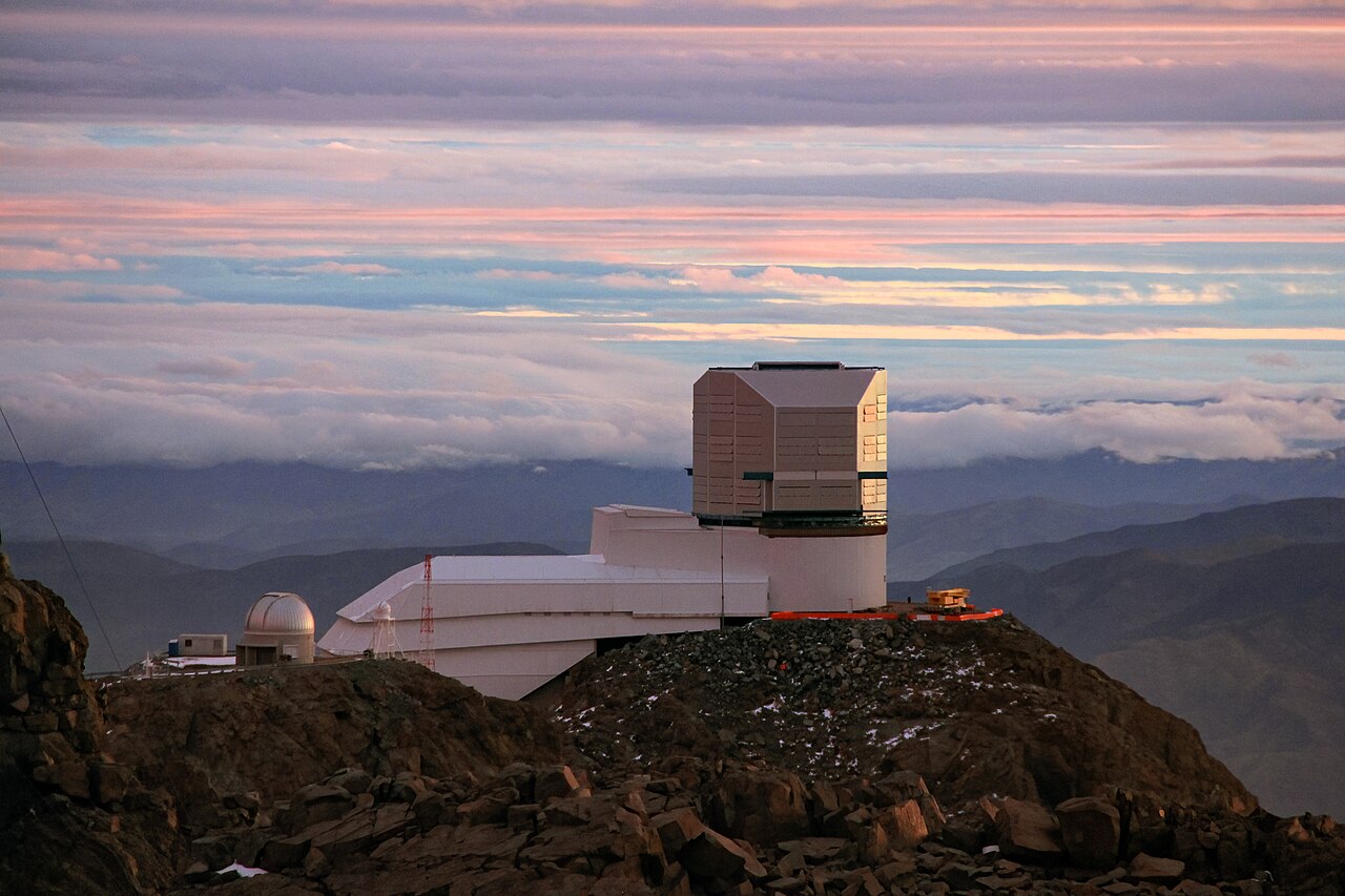
Vera C. Rubin Observatory began LSST, a ten-year survey of the sky, on the night of 29 June 2026. It records about 10 terabytes a night, some 30 petabytes over the decade, and returns to the same patch of sky close to 800 times so that what changes can be separated from what does not. Before the survey proper, the observatory released a rehearsal. That release is Data Preview 1. It holds six-band images of seven fields, about 15 square degrees in all, taken with the commissioning camera from late October 2024 to early January 2025.
The paper works with the two deepest of those fields. ECDFS and EDFS reach r-band magnitudes of 26.0 and 25.5. DeepDISC was run on them. The model finds an object, traces its outline and decides whether it is a star or a galaxy, all in one inference pass, which is a different shape from a pipeline that runs detection, deblending and classification in sequence. Its backbone is a Swin-B vision transformer, 86.8 million parameters in the backbone and 139 million in total.
Training began from a model pretrained on LSST simulations. The DP1 six-band images of the real sky were then shown to it with every weight unfrozen. The paper calls this Stage 1. Before it saw the real sky, the model scored 40.2% on galaxies and 13% on stars. After the real images, it reached 84.2% and 49.1%. Both classes improved a great deal, and the distance between them stayed where it was.
The quantity here is completeness: the share of the objects written into the ground truth that the model actually found. The 312 test tiles held 58,710 galaxies and 9,795 stars. The 84.2% and the 49.1% are what comes out when each of those two counts is taken as the denominator.
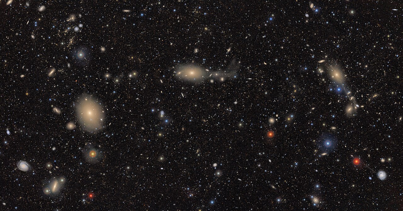
A second stage follows the one that taught detection. The backbone, the feature pyramid, the region proposal network and the detection head are all frozen, and only the classification head is trained again. The labels used here come from somewhere else. Out of a sample of 15,611 stars and galaxies in the ECDFS region, identified through spectroscopy, Gaia DR3 and photometric stellar classification, the 8,370 that fall on the Stage 1 training tiles were matched by Rubin objectId and carried over: 6,151 galaxies and 2,219 stars. With 961 synthetic sources added, 9,331 objects tuned the classification head. On a single NVIDIA H200, Stage 1 ran in under two hours and Stage 2 in under fifteen minutes.
What the 97.4% Does Not Count
The same paper carries another report card. Sorting the objects it had found into stars and galaxies, the model was 97.4% accurate. In the same ECDFS field, a random forest working from photometry alone (Gatto et al., 2026) was 98.5%. The difference is 1.1 percentage points. Set those two numbers side by side and the new deep learning model looks to have all but caught up with the established method.
But the two scores count different things. The denominator of completeness is every object written into the ground truth. The denominator of accuracy is the objects the model found. If half the stars drop out at the detection step, sorting only the remaining half correctly still produces a high accuracy. The missed stars are not even recorded as wrong answers. They drop out of the answer sheet entirely.
The comparison carries conditions of its own. The random forest takes objects the DP1 catalogue has already detected and only classifies them. DeepDISC detects and classifies together. The paper states that the two numbers are not a one-to-one comparison. Toward the faint end, DeepDISC calls more objects stars than the random forest does, and where independent labels settle the disagreement, the random forest turns out right in most of those cases.
The 97.4% and the 98.5% were measured only on a common sample that neither classifier had seen in training. Without that line the comparison does not hold, because the labels used to tune DeepDISC's classification head come from the same study as the random forest it is being measured against. Trimming the overlap keeps one side from sitting its own exam a second time.
The paper narrows the denominator once more. The authors write that the pseudo ground truth drawn from Scarlet is neither complete nor pure. Ordinary precision and recall assume that it is both, so they penalize the model for finding a real object the catalogue does not list, and penalize it again for failing to trace a spurious annotation left behind by shredding. Classification scores were therefore computed only over detections matched one-to-one with the ground truth. Unmatched detections fall out of the calculation, and the paper says Scarlet on its own cannot tell whether such a detection is a real object or an artifact.
None of this makes the 97.4% false. But if that number is the only one left in a summary, nothing records that the same model failed to place half the stars in the ground truth under the strict criterion.
The Gap Starts in the Ground Truth
The paper does not look for the cause in the architecture. The first thing it names is the make-up of the training annotations. The 994 training tiles held 163,687 galaxy annotations and 28,346 star annotations, roughly six to one. The paper states outright that this ratio suppresses star recall.
The authors did not leave the skew alone. Weighting the star class more heavily and adding focal loss raised star completeness from 49.1% to 66.6% under the same matching protocol. They kept the unweighted model as the headline result anyway: weighting pulls the Stage 2 classification scores down, and the weight itself is tuned to the class ratio of this particular training set, so it does not transfer to another patch of sky. Still, the fact that changing nothing but how much each class counted during training moved stars by more than 17 percentage points is itself a pointer to where the gap comes from.
How those annotations were made works against stars too. They are not labels placed one by one by hand but a pseudo ground truth that combines the masks produced by Scarlet deblending with the refExtendedness flag in the DP1 catalogue. refExtendedness separates objects that look like points from objects that look extended, and its verdict blurs past i-band magnitude 24. A star is the kind of object that looks like a point, so it turns ambiguous exactly at that boundary.
Trouble shows up at the other end as well. A very bright star saturates at the center, and Scarlet breaks the single object into several pieces. Overlapping spurious annotations appear, and filtering them out shrinks the star sample one more time. The boundary blurs at the faint end and the object shatters at the bright end.
Put the two sets of study material side by side and the difference sharpens. What Stage 1 learned to find objects from was 192,033 annotations generated automatically from Scarlet masks and refExtendedness, of which stars were 14.8%. What Stage 2 learned to tell stars from galaxies with was labels whose identities had been confirmed by spectroscopy and Gaia; among the 8,370 of them matched exactly by objectId, stars were 26.5%. The second set is more than twenty times smaller, and in exchange its labels come from observations independent of the upstream deblender, with less skew. The paper does not separately measure how much of the gap between galaxies and stars comes from this difference, but it is clear that this is where the gap has to be examined.
The sky the model looked at held stars and galaxies together. The material it learned detection from held six times more galaxies, and the star entries in that material were least accurate at the faintest and the brightest ends. The 49.1% reflects the shape of that material more than it reflects the model's ability.
Change the Yardstick and the Score Changes
Score the same inference against a different rule and the number moves. The paper ran two matching methods together. The strict one asks for five conditions at once. The position has to fall within 0.5 arcseconds, the class the model assigned has to agree with the ground truth, and the overlap has to clear a floor set per class. Two more follow: the ground-truth object must not already be paired with another detection, and the detection score has to clear the threshold. The loose one groups nearby objects, pairs them one to one, and never looks at class.
Galaxies came out at 84.2% and 84.9%, almost the same under both rules. Stars split into 49.1% and 74.3%. That is 25.2 percentage points. The gap does not mean the model saw nothing in those places. It means the model saw something and then failed to meet what the strict rule demands. A good number of stars were detected and called galaxies.
The yardstick does not stop at the matching rule. Where to draw the line between a candidate and a detection is also set by people. The paper swept the cap on detections per image and the duplicate-removal threshold coarsely over validation data, then narrowed in, and fixed them at a cap of 485, a duplicate-removal threshold of 0.7 and a score threshold of 0.22. That is the point where the F1 scores of the two classes sum highest. Every completeness figure in the table below comes from above that threshold.
| Scoring rule | Galaxy completeness | Star completeness |
|---|---|---|
| Strict (class has to match too) | 84.2% | 49.1% |
| Loose (position alone counts) | 84.9% | 74.3% |
| Difference between the rules | 0.7 points | 25.2 points |
A blending score is reported alongside. The share of cases where two or more objects were lumped into one came to 14.9% (95% confidence interval 12.5 to 17.8%). The same quantity for the official DP1 catalogue that Rubin Observatory runs itself is 18.0%. The paper says only that the one is consistent with, or modestly below, the other. With the upper end of the interval at 17.8%, there is room to read the two values as overlapping.
Inside DP1 alone there is no way to know whether something that looks like one object is one object. So the paper borrowed better eyes: the CANDELS GOODS-S near-infrared catalogue from the Hubble Space Telescope. Where DP1's ECDFS sees to around r-band 26, this one looks about two magnitudes deeper. The two catalogues were cross-matched over a region not used in training, and of 34,612 clean CANDELS objects 27,438 entered the comparison, against 15,928 DP1 detections in the overlapping region. The 14.9% is the share of CANDELS pairs sitting closer together than DP1 can resolve that DeepDISC saw as one. To count what was missed, a more deeply observed set of data had to exist on the side.
The weakness in telling stars from galaxies sits in Rubin Observatory's official pipeline as well. In the DP1 source injection test the paper cites, about 20% of the deliberately injected objects came out as stars under refExtendedness, and most of those were in fact galaxies; the rate at which objects injected as stars were classified correctly as stars fell to about 50% at i-band 23.8. The problem does not belong to the deep learning model alone. The ground truth this paper used came out of that pipeline, so the model has been copying down a weakness from upstream.
What unrecognized blending costs downstream is written into the paper too. In about 12% of blended galaxies the photometry is off by 0.75 magnitudes or more, and at LSST depth the noise in shear measurement rises by about 14%. That error carries through to estimates of cosmological parameters. Research that takes the catalogue and works from it inherits the flaws upstream.
The next tasks the authors list point mostly at the data too. They want to test pretraining from images alone, without human labels, at the scale of the next release, Data Preview 2. Adding quasars as a third class beside stars and galaxies is on the list, as is swapping the backbone from Swin-B to MViTv2 for comparison. Measuring faint-end performance in absolute terms rather than by relative comparison, they add, will mean running the source injection test themselves. Before any of that, they grant that the results as they stand are tied to a pseudo ground truth.
Why Pebblous Is Watching This Paper
It is an astronomy paper, but what happened in it has a shape that data quality work runs into often. When performance has to be reported as a single number, the side that is easy to measure is the side that stays in the report. Accuracy is easy. Match the model's answers against the right ones. Completeness is hard. You have to know what the whole is before you can build the denominator, and what tells you the whole is the ground truth itself.
So when the ground truth tilts, two things happen at once. The model tilts with it, and the yardstick that would measure the tilt tilts as well. That is where this paper is honest. It reported the 49.1% instead of hiding it, and it looked for the cause in annotations of its own making. Had it not, only the 97.4% would be left.
Defect detection on a production line, reading medical images, object recognition for autonomous driving: the same structure repeats. A class that appears rarely is thinly represented in the training data, a thinly represented class gets missed more often, and what is missed does not show up in accuracy. The miss never comes back as a number, so nothing ever prompts the fix.
There are three questions to ask when a model's report card arrives. What is the denominator of the number being reported? How many of each class are in the ground truth? And where does the tool that built it get weak? All three have to be answered before anyone touches the model, and the third is usually the last to open. This paper is a rare case of the third being written into the body.
It is not as though there is no way to answer. What this paper did to measure blending is the example. A value that cannot be checked inside its own data was checked against external data observed more deeply. On the ground, that place is taken by a full-inspection sample, re-labeled records, or readings from a different sensor. All of them are expensive. So they are usually skipped, and where they are skipped, accuracy is what remains.
Thank you for reading this far. The full paper is on arXiv, and the specifications and release scope of Data Preview 1 are in Rubin Observatory's documentation. If you have your own experience of what would have to change on a team for completeness, rather than accuracy, to go on the first line of a report, we would be glad to hear it.
References
Academic
- 1.Yadav, P., Ejjagiri, Y. S., Liu, X., Merz, G., & the LSST Dark Energy Science Collaboration (2026-10-07). "DeepDISC on LSST Data Preview 1: Scene-Level Detection, Deblending, and Star/Galaxy Classification in the ECDFS and EDFS Fields." arXiv:2610.10986 [astro-ph.IM].
- 2.NSF–DOE Vera C. Rubin Observatory / LSST Dark Energy Science Collaboration (2026). "The Vera C. Rubin Observatory Data Preview 1." arXiv:2603.23786.
Official Documents
- 3.Vera C. Rubin Observatory. "Rubin Observatory Data Preview 1 Documentation." (DP1 observing period, fields and bands)
- 4.Vera C. Rubin Observatory. "Legacy Survey of Space and Time (LSST)." (10TB per night, 30PB in total, about 800 revisits)
- 5.Rubin Observatory (2026-06-30). "Action! NSF–DOE Vera C. Rubin Observatory Begins Capturing the Greatest Cosmic Movie Ever Made." (start of LSST survey operations)