Executive Summary
A paper posted to arXiv on August 24 pulled 24 anomalous objects out of 373,646 periodic variable stars. The catalog is the one the ASAS-SN survey has been building, and the authors are researchers at Charles University and Ohio State. Eighteen of the 24 have never been reported as unusual in the literature. The light curves were not examined by a person. A multimodal agent did the looking, and it opened about 1 percent of the catalog.
The budget arithmetic printed next to the discovery list is the part worth lingering on. The authors worked out what the same 5,100-label budget would have bought if it had been spent straight down the initial outlier ranking. The answer is 53 of the final 177 objects, roughly 30 percent. The lowest-ranked anomaly sat near position 350,000, and walking down the list far enough to reach it would have taken about 70 times the budget.
For anyone who works with data, this does not read as an astronomy story alone. The choice of what to label first set the reach of the search rather than the accuracy of a model. And because the reviewer was an agent, the paper has to say what it takes to audit those verdicts, which it does in some detail.
Key Figures
Source: Pešta & Ting (2026), arXiv:2608.23688, abstract and Sections IV and V
5,100
Stars actually labeled
About 1% of the 373,646 in the sample
3 hours · $40
Cost of the whole pipeline
51 iterations plus the five-agent review
30%
Recovery from the initial ranking
53 of 177 objects at the same budget
70×
Budget needed for the last anomaly
It started near rank 350,000
Only 5,100 of 370,000 Were Looked At
Picking the odd star out of a variable-star catalog has always been eye work. Someone pages through light curves, the plots that show how a star's brightness rises and falls over time, and pulls out the ones that look wrong. A few thousand plots is a manageable afternoon. The catalogs that survey telescopes now build on their own run to hundreds of thousands.
The obvious objection is to point an automated outlier detector at the pile, and the paper answers it in the introduction. When Etsebeth and colleagues (2024) ran isolation forests over roughly 4 million galaxy images from DECaLS, 1,763 of the top 2,000 candidates turned out to be instrumental artifacts or masked sources, with only a single scientifically interesting anomaly in that initial ranking. An algorithm that looks for outliers finds broken data along with rare astrophysics, and separating the two lands back on a human desk.
Milan Pešta and Yuan-Sen Ting handed that desk to multimodal agents. Their sample is 373,646 periodic variables drawn from ASAS-SN Sky Patrol V2.0, cross-matched against the VSX catalog of variable stars and filtered on epoch count and magnitude range. The model doing the review is Gemini 3 Flash, and what each agent receives is a phase-folded light-curve image plus a short metadata block: period, amplitude, and the VSX class name. No object name, no sky coordinates. The class name itself was overridable, so an agent that disagreed with VSX after looking at the plot could write its own classification instead.

After 51 iterations, 5,100 stars carried labels, about 1 percent of the sample. The run took roughly 3 hours and about $40 in API calls. It returned 24 anomalies and 153 potentially interesting objects worth follow-up, and 18 of the 24 anomalies had never been flagged as unusual before.
How many days the same job would have taken a person is a number the paper never estimates. What the authors did measure themselves against is not a human but another machine, specifically the ordinary approach of ranking by outlier score and labeling nothing. That comparison produced the most practically useful figure in the paper.
Every Label Rewrites the Ranking
The pipeline starts from a picture rather than a number. Each light curve is folded on its period and rendered as a 518 by 518 pixel image with the axes and tick labels stripped away. That shape-only image goes through DINOv2 ViT-g/14 and comes out as a 1,536-dimensional vector. The model was never fine-tuned on astronomical data, and yet the embedding space separated the light curves by variability class on its own.
The initial ranking comes next. The 26 VSX classes with more than a thousand members, plus one catch-all group for everything else, each got their own isolation forest, 27 in total, and every star received an outlier score within its class. Train a single forest across the whole sample and the rare classes come out wholesale as outliers. Fitting one per class moves the line between ordinary and strange inside the class rather than across the catalog.
From there the loop turns. In each round an agent independently reviews the top 100 unlabeled candidates and assigns 0 for not interesting, 1 for potentially interesting, or 2 for anomalous. Those labels propagate through the embedding space to any neighbor whose cosine similarity exceeds 0.90, which reshuffles the ranking for the next round. To keep the search from burrowing into the neighborhoods it has already found, the authors capped the number of neighbor-elevated candidates reviewed in each iteration at half the batch. It is the classic active learning structure in which expert labels update the ranker, with only the identity of the labeler changed.
The word agent here does not mean a system that calls tools or plans its own work. A footnote in the paper defines it as an independently prompted instance of a multimodal LLM acting as an automated annotator, and adds that the agents are deliberately minimal, with no memory across evaluations, no access to external tools, and no ability to plan their own actions. One image and one prompt are the whole evidence base for a verdict.
After 50 rounds, the 51st behaves differently. The 5,000 accumulated labels train a logistic regression classifier that rescores the entire unlabeled pool, and the top 100 with anomaly probability above 0.90 go to the agents as one final batch. Similarity propagation only searches near what has already been seen, so pulling in distant candidates required one pass that looked at everything again.
Reordering the Queue Surfaced the Other 70%
The reason to run a loop at all is that the labeling budget is finite. If you can look at 5,100 stars, which 5,100 do you look at? The most common answer is the 5,100 with the highest outlier scores. The authors graded that answer. They traced back where each star in the final catalog had sat in the initial ranking, and computed what a budget spent strictly in rank order would have brought home.
Of the 24 anomalies, 10 were inside the first 5,100, which is 42 percent. Of the 153 potentially interesting objects, 43 were, which is 28 percent. Put the two categories together and it is 53 out of 177, roughly 30 percent. The other 70 percent are stars that a rank-ordered walk would never have reached before the budget ran out.
The extreme case is CSS_J163724.5+181022. This star started near rank 350,000, essentially at the bottom of the catalog. Walking down in order to reach it would have taken not 5,100 labels but about 70 times that. What actually surfaced it was the logistic regression in iteration 51. Similarity propagation never got there, and the star appeared only once the accumulated labels were used to rescore the whole pool.
Without that final pass the catalog would have been shorter. By the end of the 50 active learning rounds, about 71 percent of the anomalies and 81 percent of the potentially interesting objects had been found, and the rest came from the logistic regression step, which added 7 anomalies and 29 potentially interesting objects on its own. Even among the 9 stars that all five agents unanimously called anomalies, two lay outside the initial budget. Y Leo sat at rank 6,942 and was pulled up by neighbor label propagation, and CSS_J085817.6−075719 sat at rank 250,222 and was caught by that last logistic regression.
Whether the answer is simply a bigger budget, the authors think not. They point back to the galaxy-image study cited earlier, where the anomaly yield fell off sharply beyond 6,000 labeled samples. Active learning rarely needs more than a few thousand labels, and past that point the natural direction for scaling is across other data sets rather than deeper into the same one. Fixing the order and buying more of it are not the same move.
Nothing about the model changed here. The embeddings are the same and so are the isolation forests. What changed is the order of labeling, and that order set the reach of the search. Treat a labeling budget purely as a question of how much accuracy it buys and this difference stays invisible. The same budget also decides how far down the catalog you are able to go.
A Star Erupting for Over Two Decades
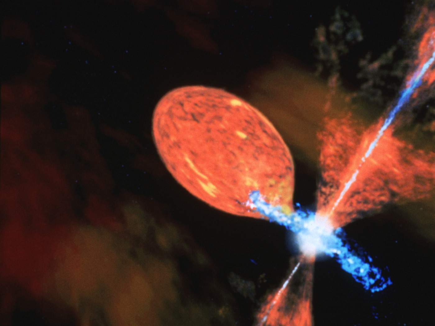
What kind of stars turned up says something about the pipeline too. The most striking is ASAS J174600−2321.3, a symbiotic nova. It has a period of 1011.5 days and pairs a white dwarf with a late M giant, and while the white dwarf works through a slow nova outburst the giant periodically occults it. Two observational reports from 2015 identified the system as an eclipsing symbiotic binary in outburst, and the later of the two read a slight drop in mean brightness as a sign that the eruption had begun to subside. Nearly a decade later, this data shows the white dwarf still in outburst. Counted from the start of the eruption, that run now exceeds two decades, which is how the paper's abstract and conclusions describe it.
The rest of the catalog is just as distinct. By the authors' own classification, the 24 anomalies break down as 10 EA-type eclipsing binaries with extremely deep primary eclipses, 7 contact binaries, 3 RRab variables, 2 Cepheids in the high-amplitude tail of their classes, one deeply eclipsing nova-like system, and the symbiotic nova above. Most of the eclipsing binaries dim by 4.02 to 4.82 magnitudes at primary minimum, a drop of 97 to 99 percent in flux. The seven contact binaries have periods of 0.27 to 0.46 days, unremarkable for the class, but amplitudes far out in the tail, which points to near-equal-mass systems in deep contact seen at high inclination. Some may be close to filling their outer critical Roche lobes, at which point rapid merger becomes possible, and that makes them high-priority follow-up targets.
Six of the 24 were already on record in the literature as unusual. The authors read those six as validation rather than failure. The agents were given neither object names nor coordinates, so they had no way to consult the literature, and recovering known peculiar objects under that constraint is independent evidence that the pipeline works.
What Audits an Agent's Verdict
When the reviewer is not a person, the review record changes character. Human labelers come with familiar yardsticks: inter-annotator agreement, re-review rates, the distribution of error types. Agents have no settled equivalent yet. What this paper puts in that place is three layers.
The first is the structure of the prompt itself. The instruction each agent receives is a 1,460-word fixed procedure in eight steps. It starts with visual inspection, moves through data quality and phase-folding checks, amplitude estimation, classification, extreme-parameter flagging, and scoring, then in step seven has the agent re-examine its own judgments before returning a structured JSON response. The rules are deliberately conservative. Data quality problems are assumed present until clear evidence overturns them, and any candidate that fails the quality and folding checks scores zero, full stop. The path by which an observational artifact gets promoted to an anomaly is closed off by construction.
The second is the consensus review. The 276 sources that scored 1 or higher in the single-agent stage went to five independent agents for re-evaluation, with the final label set by majority vote and ties broken in favor of the lower relevance class. The result is the table below.
| Single-agent verdict | Consensus: anomaly | Consensus: interesting | Consensus: not interesting |
|---|---|---|---|
| Anomaly, 43 | 20 | 9 | 14 |
| Potentially interesting, 233 | 4 | 144 | 85 |
| Total, 276 | 24 | 153 | 99 |
Ninety-nine of the 276, or 36 percent, dropped to not interesting. A single agent working alone over-flagged more than one case in three. That demotion roughly doubled the purity of the final anomaly sample, and the extra compute it took came to about 25 percent of the total. As the price of a second review pass, that is cheap.
The demotions were also not spread evenly. Broken out by class, EA-type eclipsing binaries had the lowest demotion rate at 0.24, while EB-type eclipsing binaries came in at 0.64, semiregular variables at 0.67, and rotating variables at 0.75. The reasons are legible. EB-type systems were mostly misclassified as contact binaries, which meant their periods and amplitudes were scored against that class's tighter ranges, making ordinary values look strange. Rotating and semiregular variables have messy light curves to begin with, so estimating amplitudes and spotting quality problems was harder. The errors clustered by class instead of scattering at random, and that kind of concentration does not show up when labels are inspected one at a time.
Sometimes the input was the problem more than the judgment. AQ Ind is an eclipsing binary with a 4.34-magnitude primary eclipse, but the arbitrary phase zero-point split that eclipse into two sparse streaks at the edges of the image the agents received. Three of the five read the streaks as a data quality problem and the majority vote came out at zero. RW Tri was pushed into the dwarf nova bucket because the prompt's class list had no nova-like category at all. How the plot is drawn and which options are written into the prompt ride straight into the verdict.
The third layer is the record. The full reasoning chains from all five agents were preserved, and the spread across their scores doubles as a confidence measure. The paper describes this design as ensuring that each labeling decision remains fully auditable. An appendix counts the vocabulary that appears in the rationales for each verdict, finding "exceeding" in 91.7 percent of the anomaly rationales, and "quality" in 78.8 percent and "standard" in 72.7 percent of the demotions. The diagnostic flags the agents raised split along the same line. All 24 final anomalies triggered the extreme-amplitude flag and none raised a data quality flag, while among the 99 demoted sources data quality issues appeared in 56.6 percent and outlier-dominated in 51.5 percent. It is a setup that lets you check after the fact whether what the agents said and what they flagged point the same way.
All three layers, though, only guard against over-flagging. A consensus review cannot revive a star that the single-agent stage never flagged even once. The authors note that when the priority is completeness rather than purity, one stronger agent may be needed instead of five weaker ones, and they concede that they have no record of the anomalies the pipeline failed to recover among the 373,646. A verdict that was never written down cannot be audited.
Where the labeling budget goes first sets the reach of discovery rather than the accuracy of the model. And when the reviewer is an agent, the object of quality control shifts from the verdict to the way the verdict is recorded. The authors do not see this staying at laboratory scale. They include a calculation that on an LSST stream delivering 1 million to 10 million alerts a night, a labeling budget of 10,000 sources would run the same structure for under $100 per night. The catalog and the code are published on GitHub.